Microsoft Excel is a go-to tool if you’re working with data. Starting from simple calculations to building reports, Excel has it all covered. Knowing Excel has become a necessity in today’s times. Organizations rely on Excel for storing and analyzing their data. This article on MS Excel interview questions and answers will cover the top 50 questions that could be asked in an Excel interview.
So, let’s start with our beginner level Excel interview questions.
Watch the video below on Excel interview questions and answers that covers all the basic, intermediate and advanced interview questions that are frequently asked.
Beginner Level Excel Interview Questions
We will start with a set of Excel interview questions aimed at the beginners.
1. What is a cell address in Excel?
A cell address is used to identify a particular cell on a worksheet. It is denoted by a combination of the respective column letter and a row number.
As shown above, the highlighted cell belongs to the column ‘D’ and row 5, so the cell address is read as D5.

2. What do you mean by Relative cell referencing and Absolute cell referencing in MS Excel?
Relative cell referencing |
Absolute cell referencing |
In Relative referencing, there is a change when copying a formula from one cell to another cell with respect to the destination. cells’ address |
Meanwhile, there is no change in Absolute cell referencing when a formula is copied, irrespective of the cell’s destination. |
|
This type of referencing is there by default. Relative cell referencing doesn’t require a dollar sign in the formula. |
If you don’t want a change in the formula when it’s copied across cells, then absolute referencing requires you to add a dollar sign before and after the column and row address. |
 |
 |
3. How do you freeze panes in Excel?
Freeze panes keep the rows and columns visible while scrolling through a worksheet. To freeze panes, select the View tab and go to Freeze Panes.

If you are looking to freeze the first two columns of a dataset, select the 3rd column, and click ‘Freeze Panes’. A thick grey border indicates this.

4. How can you restrict someone from copying a cell from your worksheet?
1. First, choose the data you want to protect.

2. Hit Ctrl + Shift + F. The Format Cells tab appears. Go to the Protection tab. Check Locked and click OK.

3. Next, go to the Review tab and select Protect Sheet. Enter the password to protect the sheet.
Let’s now move onto our next question on our list of Excel interview questions.
5. How is a Formula different from a Function in Excel?
The formula is like an equation in Excel, the user types in that. It can be any type of calculation depending on the user’s choice. |
Whereas, a function in Excel is a predefined calculation which is in-built in Excel. |
|
Manually typing out a formula every time you need to perform a calculation, consumes more time. Ex: = A1+A2+A3 |
However, performing calculations becomes more comfortable and faster while working with functions. Ex: = SUM(A1:A3) |
Now, let’s head to our next question in our list of Excel interview questions.
6. Mention the order of operations used in Excel while evaluating formulas.
The order of operations in Excel is referred to as PEDMAS. Shown below is the order of precedence while performing an Excel operation.
- Parentheses
- Exponentiation
- Division/Multiplication
- Addition
- Subtraction
As seen above, first, the data in the parentheses is operated, followed by the exponentiation operation. After that, it can be either the division or multiplication operations. The result is then added and finally subtracted to give the final result.
Let’s look at an example of the PEMDAS precedence in the next question on our Excel interview questions list.
7. How will you write the formula for the following? - Multiply the value in cell A1 by 10, add the result by 5, and divide it by 2.
To write a formula for the above-stated question, we have to follow the PEDMAS Precedence. The correct answer is ((A1*10)+5)/2.
Answers such as =A1*10+5/2 and =(A1*10)+5/2 are not correct. We must put parentheses brackets after a particular operation.
The output will look like this:

8. What is the difference between count, counta, and countblank?
The count function is very often used in Excel. Here, let’s look at the difference between count, and it’s variants - counta and countblank.
1. COUNT
It counts the number of cells that contain numeric values only. Cells that have string values, special characters, and blank cells will not be counted. Shown below is an example of the count function.

2. COUNTA
It counts the number of cells that contain any form of content. Cells that have string values, special characters, and numeric values will be counted. However, a blank cell will not be counted. Shown below is an example of the counta function.

3. COUNTBLANK
As the name suggests, it counts the number of blank cells only. Cells that have content will not be taken into consideration. Shown below is an example of the countblank function.

9. What is the shortcut to add a filter to a table?
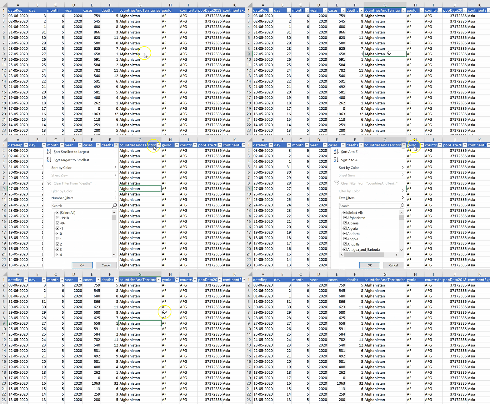
The filter mechanism is used when you want to display only specific data from the entire dataset. By doing so, there is no change being made to the data. The shortcut to add a filter to a table is Ctrl+Shift+L.
10. How do you create a hyperlink in Excel?
Hyperlinks are used to navigate between worksheets and files/websites. To create a hyperlink, the shortcut used is Ctrl+K.
The ‘Insert Hyperlink’ box appears. Enter the address and the text to display. Here, we are directed to the Amazon Website.

11. How can we merge multiple cells text strings in a cell?
To merge text strings present in multiple cells into one cell, you can use the CONCATENATE(). Shown below is an example of the concatenate function.

Another way of combining cell values is by using the “&” operator, as shown below:

Let’s now move onto the next question on our Excel interview questions list.
12. How can you split a column into 2 or more columns?
You can split a column into 2 or more columns by following the below steps:
1. Select the cell that you want to split. Then, navigate to the Data tab, after that, select Text to Columns.

2. Select the delimiter.

3. Choose the column data format and select the destination you want to display the split.

4. The final output will look like below where the text is split into multiple columns.

13. What is the use of VLOOKUP and how do we use it?
The function VLOOKUP in Excel is used to look up information in a table and extract the corresponding data.
Syntax: VLOOKUP (value, table, col_index, [range_lookup])
value - Indicates the data that you are looking for in the first column of a table.
table - Refers to the set of data (table) from which you have to retrieve the above value.
col_index - Refers to the column in the table from where you are to retrieve the value.
range_lookup - FALSE = exact match [optional] TRUE = approximate match (default).
Shown below is an example of the VLOOKUP function. We are to find the Product related to the Customer Name – “Richard”.

14. How is VLOOKUP different from the LOOKUP function?
VLOOKUP |
|
|
VLOOKUP lets the user look for a value in the left-most column of a table. It then returns the value in a left-to-right way. It is not very easy to use as compared to the LOOKUP function. |
Meanwhile, the LOOKUP function enables the user to look for data in a row/column. It returns the value in another row/column. It is easier and can also be used to replace the VLOOKUP function. |
15. How many report formats are available in Excel?
There are three report formats available in Excel; they are:
- Compact Form
- Outline Form
- Tabular Form
16. How does the IF() function in Excel work?
In Excel, the IF() function performs a logical test. It returns a value if the test evaluates to true and another value if the test result is false. It returns the value depending on whether the condition is valid for the entire selected range.
Let’s look at the below example:

As seen above, the IF function returns “Record is Valid” if age is greater than 20, and the salary should be greater than $40000. Else, it will return “Record is Invalid”. Here the final answer will be “Record is Valid” as the entire selected range qualifies both the conditions.
17. How do we use the SUMIF() function in Excel?
The SUMIF() function adds the cell values specified by a given condition or criteria. Given below is an example of the sumif function.

As seen above, the costs corresponding to the years 2010 are added as per the given criteria.
18. Using the COVID data, find the number of days in which the number of deaths in Italy has been greater than 200.
To perform this operation, we can use the COUNTIFS() function. The dataset we will be using is shown below:

The COUNTIFS() function we use is - =COUNTIFS(G2:G35777,"Italy",E2:E35777,">200")
19. What is a Pivot Table?
A pivot table is like a summary table of the dataset that enables you to create reports and analyze trends. They are useful when you have long rows or columns that hold values you need to track.
To create a pivot table, first, go to the Insert tab and select the ‘PivotTable’ option.

Select the table or the range and choose where you want to place the pivot table.

Drag the fields you wish to show in the pivot table. Here we have created a pivot table using the Coronavirus data.

20. Create a drop-down list in Excel.
This can be done by using the ‘Data Validation’ option present in the Data tab.

In the example below, we have created a list based on the city column of the dataset.

21. How do we apply advanced filters in Excel?
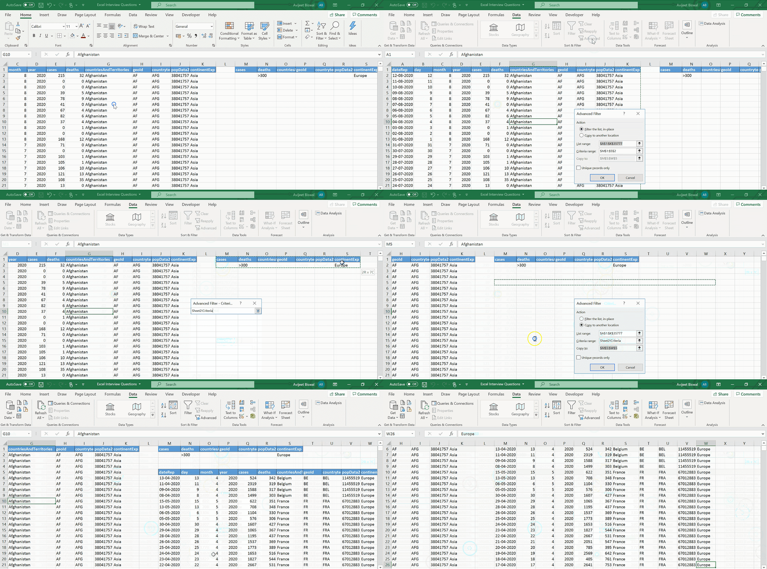
To apply advanced filters, use the Advanced Filter option present in the Data tab. Select where you want to filter the table. Choose the ‘list range’ and the ‘criteria range’ that has the conditions based on which you would like to filter the table.

The below example shows how to apply advanced filters.
22. Using the below-given sales data, highlight those cells where total sales > $5000.
Here, conditional formatting is used to highlight cells based on the criteria.

1. Select ‘Conditional Formatting’ from the home tab and under Highlight Cells Rules, choose ‘Greater Than option’.

2. Provide the condition and choose the color for the cells to be highlighted.


23. Using the given table, explain how the index-match function works in Excel.
Here, we will write an index-match function to find the city to which Andrew belongs to from the below table.

Here is how you can use the Index-Match function to get the result.

24. How do you find duplicate values in a column?
To find duplicate values in a column, you can either use Conditional Formatting or the COUNTIF() function.
1. Conditional Formatting
First, go to the Home tab, then under Conditional Formatting, select ‘Highlight Cells Rules’. Then choose ‘Duplicate Values’.

Below, we have highlighted the cells in the ‘Name’ column that have been repeated.
2. COUNTIF()
You can write a COUNTIF() function to check if the values in a particular column are repeated.

In the below example, we are fetching the duplicate names using the COUNTIF() function.
25. How can you remove duplicate values in a range of cells?
1. To delete duplicate values in a column, select the highlighted cells, and press the delete button. After deleting the values, go to the ‘Conditional Formatting’ option present in the Home tab. Choose ‘Clear Rules’ to remove the rules from the sheet.

2. You can also delete duplicate values by selecting the ‘Remove Duplicates’ option under Data Tools present in the Data tab.
Moving forward, let’s have a look at the intermediate level of Excel interview questions.
Intermediate Level Excel Interview Questions
26. What are the wildcards available in Excel?
Wildcards only work with text data. Excel has three wildcards.
1. * (Asterisk)
This refers to any number of characters.
The example stated below filters the customers whose name ends with “a”.
For that, we use “*a”.

2. ? (Question mark)
It represents one single character.
The example below shows how to filter a particular customer name.

3. ~ (Tilde)
It is used to identify a wildcard character (~, *, ?) in the text.
In the following example, we are filtering How?* using the tilde (~) symbol.

27. What is Data Validation? Illustrate with an example.
Data Validation restricts the type of values that a user can enter into a particular cell or a range of cells.
In the Data tab, select the ‘Data Validation’ option present under Data Tools.

Select the kind of data validation you want to apply.

In the following example, we have applied data validation to the ‘Name’ column to accept only text values. If you enter something other than a text, it will throw an error.

28. Given below is a student table. Write a function to add pass/fail to the results column based on the following criteria.
If student marks > 60 and attendance > 75%, then pass else the student fails.

You can use the IF() function and check with an AND condition to fill in the results column.

29. Calculate your age in years from the current date.
Use the YEARFRAC() or DATEDIF() function to return the number of whole days between start_date and end_date
- YEARFRAC()

- DATEDIF()

Learn best business analysis techniques by Purdue University, IB and EY experts. Sign-up for our Post Graduate Program in Business Analysis TODAY!
30. How are nested IF statements used in Excel?
The function IF() can be nested when we have multiple conditions to meet. The FALSE value in the first IF function is replaced by another IF function to make a further test.
Below, using nested IF statements, we are categorizing results based on the marks.

31. From the below table, find the descriptive statistics of the columns using the Data Analysis ToolPak in Excel.

Add the Analysis ToolPak from Options ----> Add-ins ----> Analysis ToolPak.
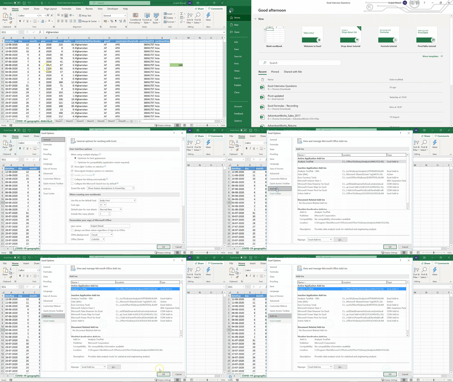
Click on the Data Analysis option in the Data tab. Choose Descriptive Statistics.

Below is the summary table for the columns and their respective statistical measures.

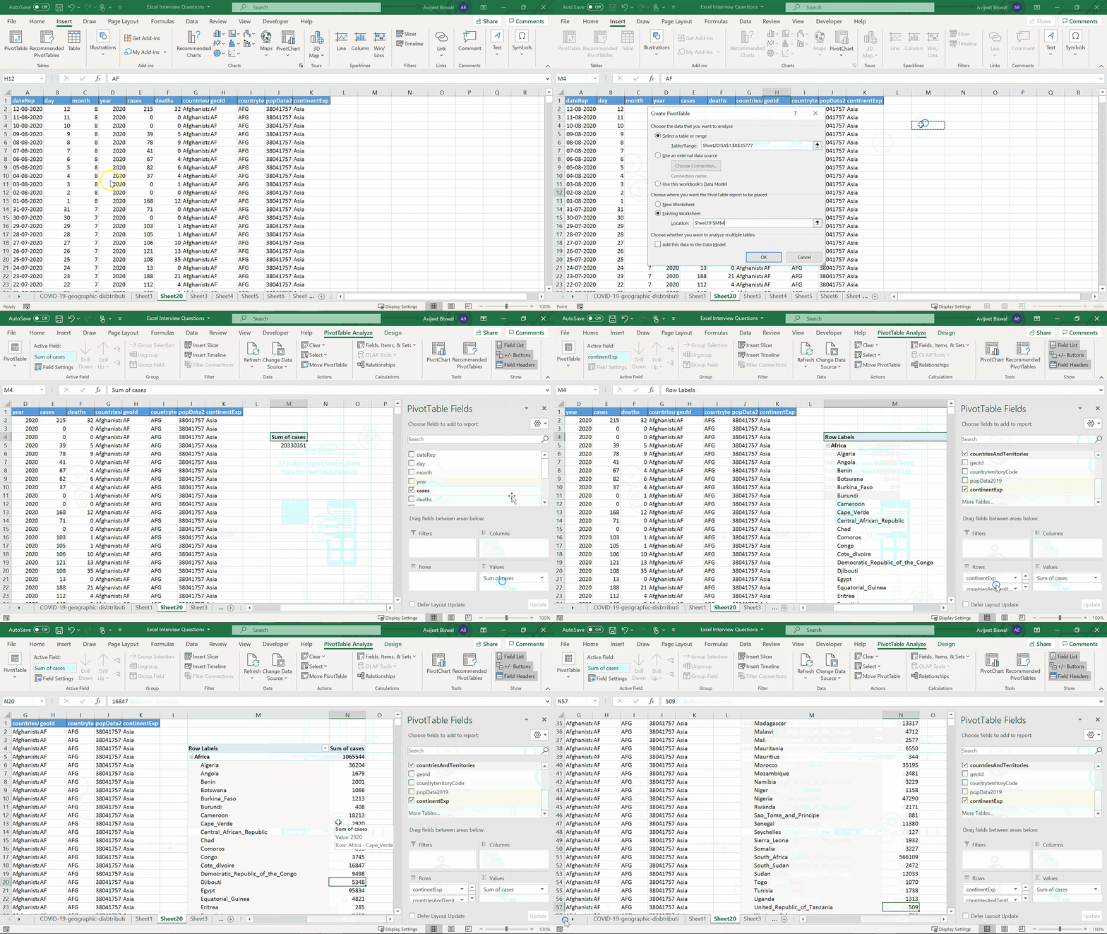
32. Using the Coronavirus dataset, create a pivot table to find the total cases in each country belonging to their respective continents.
First, drag the continent and country columns into rows. After that, drag the cases column on to the values section.
33. How do you provide Dynamic Range in ‘Data Source’ of Pivot Tables?
Dynamic Range in the data source of pivot tables is used to make your pivot table dynamic to adjust to new data when refreshed automatically.
Create a Named table to provide a dynamic range. Go to the Insert tab and select Table.

Under Table Design, give a name to the table.

Become job-ready with a globally recognized Business Analyst Certification Course. Sign-up today and enrich your career.
34. Is it possible to create a Pivot Table using multiple sources of data?
Yes, you can create a pivot table from multiple worksheets. For this, there must be a common row in both the tables. This will act as the Primary key for the first table and Foreign key for the second table. Create a relationship between the tables and then build the pivot table.
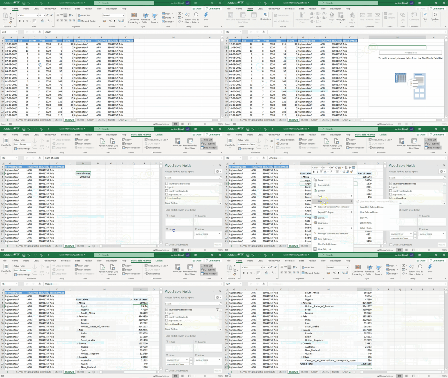
35. Create a pivot table to find the top three countries from each continent based on the total cases using COVID data.
- Create a pivot table using the coronavirus dataset by dragging sales into values.
- Place the continent and country columns into rows.
- Filter the table by selecting ‘Top 3’.
Below is the sequence of steps to follow.
36. How do you create a column in a pivot table?
For this, you have to go to the PivotTable Analyze tab and select ‘Fields, Items & Sets’ option. Under that, you need to click ‘Calculate Field’ to create a new column.

The Insert Calculated Field box appears. Give a name to the column and insert the formula by selecting the existing columns from the pivot table. Click Add ----> OK to create the column.

37. How does a Slicer work in Excel?
To filter data in a Pivot table, we can use slicers.
- To create a slicer, go to the Insert tab, and select Slicer present under Filter.
- Then, select the list of fields for which you want to create slicers.
In the below example, we have created two slicers (months, countries, and territory) to filter the pivot table.

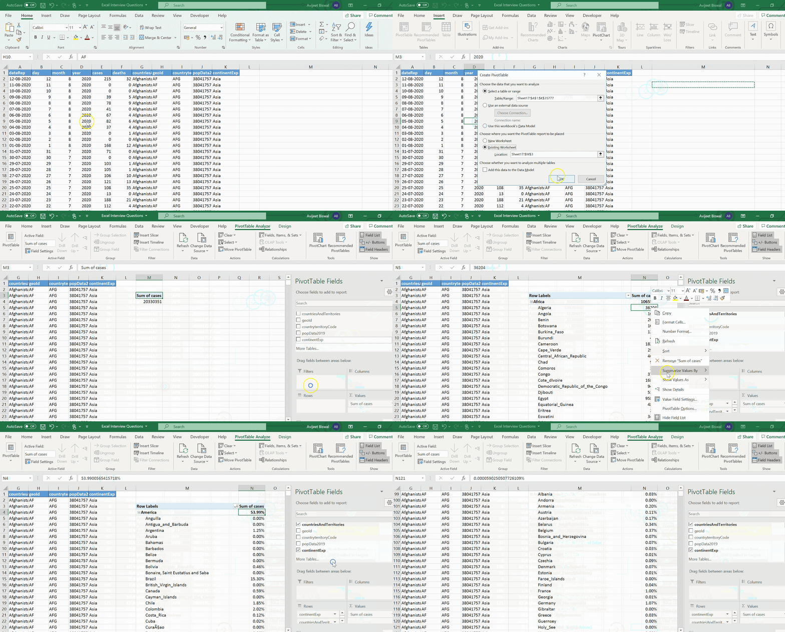
38. Use the coronavirus dataset to find the percentage contribution of each country and continent to the total cases?
- Create the pivot table to show the total cases by country and continent.
- Right-click on the sum of cases column and under Show Value As, select “% of Grand Total.”
39. How do you create a pivot chart in Excel?
- To create a pivot chart, first, we need to create a pivot table.

- Go to the Insert tab next and select the ‘Pivot Chart’ option. Choose a suitable chart to represent your pivot table data.

Accelerate your career with our Post Graduate Program in Business Analytics in partnership with Carlson School of Management. Enroll and start learning!
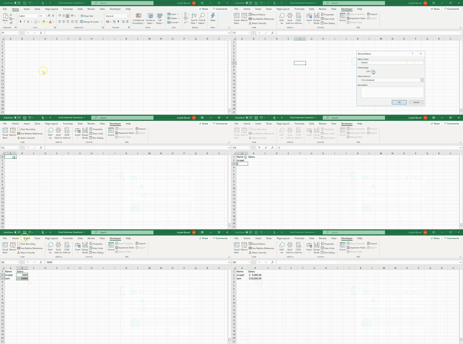
40. What are macros in Excel? Create a macro to automate a task.
Macro is a program that resides within the Excel file. The use of it is to automate repetitive tasks that you would like to perform in Excel.
To record a macro, you can either go to the Developer tab and click on Record Macro or access it from the View tab.

Now that we are done with the intermediate level of the Excel interview questions, let’s move on to the advanced level of Excel interview questions.
Advanced Level Excel Interview Questions
41. What is the What-If Analysis in Excel?
The What-If Analysis in Excel is a powerful tool to perform complex mathematical calculations, experiment with data, and try out different scenarios.
Consider the following example:
If you get $10,000 worth of sales over the next few months, how much profit can you expect?”

Such scenarios can be solved using the What-If Analysis.
Go to the Data tab and click on What-If Analysis present under Forecast.
Scenario Manager is used for a comparison of different scenarios.
The Goal Seek performs reverse calculations.
The Data Table is used for sensitivity analysis.
To learn more about how What-If analysis works, click on this link: “IQ video link”
42. What is the difference between a function and a subroutine in VBA?
Functions |
Subroutines |
A function is responsible for returning the value of the task it is performing. |
Meanwhile, subroutines don’t return the value of the task it is performing. |
They are called by a variable. |
They can be recalled from anywhere in the program, in multiple types. |
Functions are used as it is in spreadsheets as formulas. |
Subroutines are not used directly in spreadsheets as formulas. |
Functions are used to carry out repetitive tasks, and it, in turn, returns a value. |
Users are required to insert a value in the desired cell before fetching the result of the subroutine. |
43. What is the difference between ThisWorkbook and ActiveWorkbook in VBA?
ThisWorkbook |
ActiveWorkbook |
ThisWorkbook indicates the name of the workbook where the code is running from. |
As the name suggests, ActiveWorkbook is the workbook that is presently active from the various open workbooks. |
 |
 |
44. How will you pass arguments to VBA Function?
Arguments can be passed to a VBA function as a reference or as a value.
Below is an example to illustrate both the usages.
Dim x As Integer
x = 10
MsgBox Triple(x)
MsgBox x

If you run the cells by passing the values as a reference, it will display 40 both the times. When we pass arguments by reference, we are referencing the original value. The original value of x is changed in the function.
When we pass the arguments by value, we are passing a copy to the function. The original value is not changed. Hence, the second MsgBox will display the original value 10.
45. How do you find the last row and column in VBA?
To find the last row, use the below lines code in the VBA module:
Sub FindingLastRow()
Dim lastRow As Long
lastRow = ActiveSheet.Cells.SpecialCells(xlLastCell).Row
MsgBox (lastRow)
End Sub
To find the last column, use the below lines code in the VBA module:
Sub FindingLastColumn()
Dim lastRow As Long
lastColumn = ActiveSheet.Cells.SpecialCells(xlLastCell).Column
MsgBox (lastColumn)
End Sub
Want to learn the latest business analysis skills? Sign-up for our Post Graduate Program in Business Analytics and gain the skills to excel in the business world. Start learning TODAY!
46. How do we check whether a file exists or not in a specified location?
Sub CheckFileExists()
Dim strFileName As String
Dim strFileExists As String
strFileName = “File location\file_name.xlsx”
strFileExists = Dir(strFileName)
If strFileExists = “” Then
MsgBox “The selected file doesn't exist”
Else
MsgBox “The selected file exists”
End If
End Sub
47. Explain how to debug a VBA code?
To debug a VBA code line by line, you can use the F8 key. You can also create a breakpoint to terminate the execution wherever you want.
The execution will start from the beginning of the code, and every time you press F8, it will execute the next line and continue until the end of the code. The yellow arrow and the highlighted line tells you the current point to execution.

48. Write a VBA function to calculate the area of a rectangle.
Function Area(Length As Double, Optional Width As Variant)
If IsMissing(Width) Then
Area = Length * Length
Else
Area = Length * Width
End If
End Function
49. Write a VBA function to check if a number is a prime number or not.
Sub Prime()
Dim divisors As Integer, number As Long, i As Long
divisors = 0
number = InputBox(“Enter a number”)
For i = 1 To number
If number Mod i = 0 Then
divisors = divisors + 1
End If
Next i
If divisors = 2 Then
MsgBox number & “ is a prime number”
Else
MsgBox number & “ is not a prime number”
End If
End Sub
Learn the latest tools, work on real-world projects, and attend Masterclasses from IBM and EY experts. Join our Master's program today.
50. Write a VBA code to create a bar chart with the given data.
Consider the below data that has two features. You can use the lines of code below to create a bar chart.

Once you have run the above VBA code lines, below is the bar chart you will get.

So, those were the 50 Excel interview questions that can help you crack your Excel interviews and help you in bagging your dream job.
Conclusion
Now that you know the various Excel interview questions that can be asked in an interview, you can prepare by referring to the given answers for each of these Excel interview questions. Here, we had a look at a plethora of Excel interview questions based on different levels of difficulty. Practicing Excel regularly and going through these Excel interview questions will keep you prepared for any question that is thrown at you.
To kick-start your fruitful career in Excel, enroll in Business Analytics with Excel course today!
We hope this article on Excel interview questions was useful. Do you have any questions related to this article? If so, then please put it in the comments section of the article and our experts will get back to you on that right away.
